Activity: Integrated Resistors and Capacitors: Difference between revisions
No edit summary |
|||
| Line 40: | Line 40: | ||
It is interesting to note that the sign of the temperature coefficient of <math>n^+</math> polysilicon resistors is opposite of the <math>p^+</math> polysilicon resistors. Thus, it is possible to cancel the first order temperature dependence if we replace a single resistor, <math>R</math> with a <math>n^+</math> polysilicon resistor, <math>R_N</math>, in series with a <math>p^+</math> polysilicon resistor, <math>R_P</math>, where <math>R=R_N + R_P</math>. | It is interesting to note that the sign of the temperature coefficient of <math>n^+</math> polysilicon resistors is opposite of the <math>p^+</math> polysilicon resistors. Thus, it is possible to cancel the first order temperature dependence if we replace a single resistor, <math>R</math> with a <math>n^+</math> polysilicon resistor, <math>R_N</math>, in series with a <math>p^+</math> polysilicon resistor, <math>R_P</math>, where <math>R=R_N + R_P</math>. | ||
Use the following <math>p^+</math> polysilicon resistor characteristics: | Use the following <math>p^+</math> polysilicon resistor characteristics: <math>R_\mathrm{sh} =180\mathrm{\Omega}</math>, and <math>T_C =200\mathrm{ppm/^\circ C}</math> at a nominal temperature, <math>T_\mathrm{nom} =27\mathrm{^\circ C}</math>. | ||
Verify your results using SPICE for <math>R=1\,\mathrm{k\Omega}</math> with a width of <math>w=2\,\mathrm{\mu m}</math>. Note that you need to calculate the required lengths of the resistors. | Verify your results using SPICE for <math>R=1\,\mathrm{k\Omega}</math> with a width of <math>w=2\,\mathrm{\mu m}</math>. Note that you need to calculate the required lengths of the resistors. | ||
Revision as of 11:53, 12 September 2022
Activity: Integrated Resistors and Capacitors
- Instructions: This activity is structured as a tutorial with two activities. Should you have any questions, clarifications, or issues, please contact your instructor as soon as possible.
- At the end of this activity, the student should be able to:
- Understand and observe the effects of the fabrication process on passive RC circuits.
Reading Assignment
Go over the Phillip Allen's excellent slides on resistors and inductors and capacitors. Focus on the non-idealities of integrated resistors and capacitors, and how designers can work around these non-idealities to create reliable circuits.
Modeling Integrated RC Circuits
In order to model and simulate integrated resistors and capacitors, we can create semiconductor resistor models in SPICE that contains the sheet resistance of the layer, and the temperature coefficient. Consider an n-type polysilicon resistor, with , and at a nominal temperature, . Let us create a resistor model rpoly_n:
.model rpoly_n R rsh=100 tc1=-800u tnom=27C
Instantiating a resistor using the rpoly_n model, with the appropriate width and length, as:
R1 in out rpoly_n w=2u l=20u
We can also create a MOM capacitor model, and a metal-to-substrate capacitor model using:
.model cmom C cj=50m tc1=30u tnom=27C
.model cmsub C cj=30m tc1=25u tnom=27C
Where cmom is the model name of the capacitor, cj is the capacitance density in Farads per square meter, tc1 is the first order temperature coefficient, and tnom is the nominal temperature. We can then create a subcircuit cm, so every time we instantiate cm, we are including the bottom-plate capacitance in addition to the main capacitance.
.subckt cm  top bottom sub  w=1000u l=2000u
C1		top bottom	cmom w={w} l={l}
Csub	bottom sub	cmsub w={w} l={l}
.ends
Activity 1: Resistor Temperature Correction
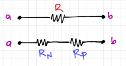
It is interesting to note that the sign of the temperature coefficient of polysilicon resistors is opposite of the polysilicon resistors. Thus, it is possible to cancel the first order temperature dependence if we replace a single resistor, with a polysilicon resistor, , in series with a polysilicon resistor, , where .
Use the following polysilicon resistor characteristics: , and at a nominal temperature, .
Verify your results using SPICE for with a width of . Note that you need to calculate the required lengths of the resistors.
Submission
Graduate and undergraduate students: submit a 1-page report showing your calculations, and a plot of the temperature characteristics of your compound resistor.
Effects of Process Variations
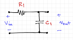
We will use SPICE to simulate the effects of process variations by allowing us to add small random changes in the sheet resistance or capacitance density of our devices. We can add random mismatch between devices by introducing small random changes to the device dimensions. We can also get a large number of samples by running the simulations repetitively using these modified device and process parameters. This is called Monte Carlo Analysis. Let us simulate the simple RC circuit in Fig. 2, and determine its corner frequency using ac analysis.
In ngspice, inside the .control block, we can define a Gaussian random number generator that takes in a nominal value, nom, the variance, var as:
define gauss(nom, var) (nom + nom*var * sgauss(0))
We can introduce mismatch by using the alter command within the .control block. This allows us to change the individual device properties. For example:
alter @R1[l] = gauss(20u, 0.01)
alter @R1[w] = gauss(2u, 0.01)

let len1 = gauss(2000u, 0.01)
alter @c.x1.c1[l] = len1
alter @c.x1.csub[l] = len1

let len2 = gauss(1000u, 0.01)
alter @c.x1.c1[w] = len2
alter @c.x1.csub[w] = len2
The altermod command, also within the .control block, let's us change the characteristics of all the devices based on a particular model. We can use this to introduce process variations to our simulations:
altermod @rpoly_n[rsh] = gauss(100, 0.01)
altermod @cmom[cj] = gauss(50m, 0.01)
altermod @cmsub[cj] = gauss(30m, 0.01)
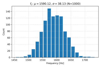
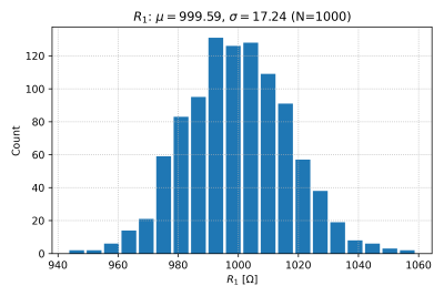
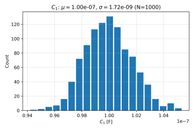
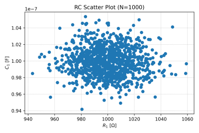
The complete SPICE file for running a Monte Carlo simulation with 1000 runs is here. The output of our SPICE file is a text file containing the We will use this Python script to run the simulation, read the SPICE output file, and plot a histogram of the corner frequency, shown in Fig. 3. The histogram of resistor and capacitor values are also shown in Figs. 4 and 5. We can also check for correlations using scatter plots, as seen in Fig. 6.
Activity 2: Monte Carlo Simulation
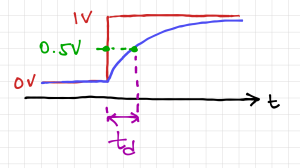
Repeat the above simulation but using a transient analysis. You are tasked to generate a histogram, with , of the low-to-high propagation delay at the output when the input is an ideal step from 0 to 1V. Note that propagation delay, , is defined as the time it takes for the output to reach 50% of its final value, as shown in Fig. 7. Feel free to edit the SPICE and Python codes given above.
Submission
Graduate and undergraduate students: submit a 1-page report explaining your approach in completing this activity. Please include your SPICE netlist, Python code, and propagation delay histogram.


