Activity: A Wideband Voltage Divider Circuit

• Activity: Simulating A Wideband Voltage Divider Circuit
• Instructions: Each activity is structured as a tutorial, and you are expected to download the netlists, run the simulation, and make sure you understand the concepts and ideas presented. Should you have any questions, clarifications, or issues, please contact your instructor as soon as possible.
  • If you are new to ngspice, please visit the Installing NGSPICE page.
• At the end of this activity, the student should be able to:

1. Run AC and transient simulations using ngspice.

A Wideband RC Voltage Divider

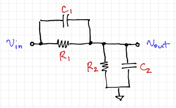
One way to build high-speed circuits with relatively large input impedances and capacitances is to use a simple RC voltage divider, as shown in the figure below. This RC divider is commonly found in 10X oscilloscope probes.

Figure 1: A wideband voltage divider circuit.

Let $Z_{1}=R_{1}\|{\frac {1}{sC_{1}}}={\frac {R_{1}}{1+sR_{1}C_{1}}}$ and similarly $Z_{2}={\frac {R_{2}}{1+sR_{2}C_{2}}}$. Thus, the output voltage can be expressed as:

$v_{out}={\frac {Z_{2}}{Z_{1}+Z_{2}}}\cdot v_{in}={\frac {R_{2}}{R_{1}+R_{2}}}\cdot {\frac {1+sR_{1}C_{1}}{1+s{\frac {R_{1}R_{2}}{R_{1}+R_{2}}}\left(C_{1}+C_{2}\right)}}\cdot v_{in}={\frac {R_{2}}{R_{1}+R_{2}}}\cdot {\frac {1+{\frac {s}{\omega _{z}}}}{1+{\frac {s}{\omega _{p}}}}}\cdot v_{in}$

Notice that we can cancel out the pole with the zero when we set $\omega _{z}=\omega _{p}$, or equivalently,

${\frac {C_{1}}{C_{1}+C_{2}}}={\frac {R_{2}}{R_{1}+R_{2}}}$

Intuitively, we can think if this as a resistive voltage divider at low frequencies, and a capacitive divider with the same ratio at high frequencies. Thus, the output voltage will simply be equal to:

$v_{out}={\frac {R_{2}}{R_{1}+R_{2}}}\cdot v_{in}$

We can then build a simple 10X oscilloscope probe circuit with an input impedance of $1\,\mathrm {M\Omega }$ and an input capacitance of $1\,\mathrm {pF}$ using $R_{1}=900\,\mathrm {k\Omega }$, $R_{2}=100\,\mathrm {k\Omega }$, $C_{1}=1.11\,\mathrm {pF}$, and $C_{2}=10\,\mathrm {pF}$. Since the pole and zero cancel each other out, the bandwidth of the probe circuit is not limited by its RC values.

Let's look at the frequency response and transient response of this circuit using ngspice.

The RC Voltage Divider Netlist

Let us start with the SPICE netlist below, where we will analyze it piece by piece. Please refer to the ngspice user manual for a more detailed description of the ngspice syntax, commands, devices, and analyses.

Line 1 is always reserved for the circuit title, and in this case, it is followed by a comment. The .options directive in line 4 instructs the simulator to save the device current data for later printing or plotting.

1 * Wideband Voltage Divider Circuit
2 * LPA 05 Aug 2020
3 
4 .options savecurrents

The next few lines describe our wideband voltage divider, composed of the resistors $R_{1}$, $R_{2}$, $C_{1}$, and $C_{2}$.

 6 R1		in out		900k
 7 R2		out 0		100k
 8 
 9 C1		in out	 	1.1111p
10 C2		out 0		10p

To examine the effects of increasing the value of $C_{1}$, we can add another circuit, but with $C_{1}=1.6\,\mathrm {pF}$.

12 * increase C1 and see what happens
13 R1a		in outa		900k
14 R2a		outa 0		100k
15 
16 C1a		in outa	 	1.6p
17 C2a		outa 0		10p

Similarly, we can add yet another circuit with $C_{1}=0.7\,\mathrm {pF}$.

19 * decrease C1 and see what happens
20 R1b		in outb		900k
21 R2b		outb 0		100k
22 
23 C1b		in outb	 	0.7p
24 C2b		outb 0		10p

We then add an input voltage, V1, that has a DC value of $1\,\mathrm {V}$, an AC value (for our ac analysis later) also equal to $1\,\mathrm {V}$, and during transient analysis, it will generate a square wave that goes from $+1\,\mathrm {V}$ to $-1\,\mathrm {V}$, no time delay, a rise and fall time of $0.1\,\mathrm {\mu s}$, a pulse width of $5\,\mathrm {\mu s}$, and a period of $10\,\mathrm {\mu s}$. The voltage source V1 is connected to the inputs of all three of our RC divider circuits.

26 * input square wave
27 V1		in 0		dc 1 ac 1 pulse(-1 1 0 0.1u 0.1u 5u 0.01m)

After describing the circuits we want to simulate, we then add a control block, which begins with the .control directive, and ends with the .endc directive. The following analyses are then queued:

• An AC Analysis is invoked by the command in line 31. The parameters instruct the simulator to calculate 10 points per decade, starting at $1\,\mathrm {Hz}$ and ends at $1\,\mathrm {GHz}$. After the simulation completes, it plots the magnitude of the output voltage of all three circuits in dB, then writes the raw data in a file called testac.dat.

• A Transient Analysis is invoked by the command in line 35, instructing the simulator to run for $30\,\mathrm {\mu s}$ with a step time of $10\,\mathrm {ns}$. And once again, plot the output voltages of the three RC voltage dividers, but this time with respect to time instead of frequency. The raw simulation data is then written to the file testtran.dat.

Try to look at the contents of these output files. We can use these files to perform more sophisticated automation, processing, analysis, and visualization using Python (or other similar languages and tools) as seen in the Using Python with NGSPICE tutorial.

29 .control
30 
31 ac dec 10 1 1G
32 plot vdb(out) vdb(outa) vdb(outb) 
33 wrdata testac.dat v(out) v(outa) v(outb)
34 
35 tran 0.01u 0.03m
36 plot v(out) v(outa) v(outb)
37 wrdata testtran.dat v(out) v(outa) v(outb)
38 
39 .endc

Finally, we end the netlist by the .end directive.

41 .end

Simulating the RC Voltage Divider

Running ngspice at the command line, and loading the netlist using source wideband_voltage_divider.sp gives us:

******
** ngspice-31 : Circuit level simulation program
** The U. C. Berkeley CAD Group
** Copyright 1985-1994, Regents of the University of California.
** Please get your ngspice manual from http://ngspice.sourceforge.net/docs.html
** Please file your bug-reports at http://ngspice.sourceforge.net/bugrep.html
******
ngspice 1 -> source wideband_voltage_divider.sp

Circuit: * wideband voltage divider circuit

Doing analysis at TEMP = 27.000000 and TNOM = 27.000000


No. of Data Rows : 91
Doing analysis at TEMP = 27.000000 and TNOM = 27.000000


Initial Transient Solution
--------------------------

Node                                   Voltage
----                                   -------
in                                          -1
out                                       -0.1
outa                                      -0.1
outb                                      -0.1
v1#branch                                3e-06


No. of Data Rows : 3041
ngspice 2 ->

The simulator will also generate two plots:

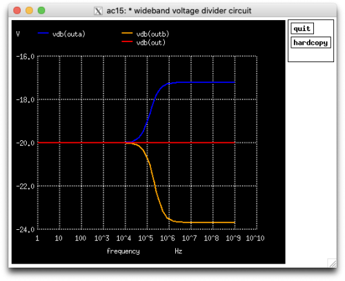
• A frequency response plot showing the output voltage as a function of frequency for all three circuits, shown in Fig. 2. Note that if the pole frequency is higher than the zero (outa), the magnitude response increases, then levels off after the pole, thus the gain at higher frequencies would be higher. The opposite is true when the pole frequency is lower than the zero. When the pole and zero perfectly cancels each other out, we get a constant gain over frequency of $20\cdot \log \left(0.1\right)=-20\,\mathrm {dB}$.

Figure 2: The RC divider magnitude response.

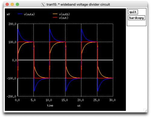
• A transient response plot, in Fig. 3. Notice that the output outa has an overshoot at high frequencies, reinforcing our observations from the frequency response plot. The opposite is again true for outb, where the high frequency components have less gain, resulting on slower rise and fall times. And again, with perfect pole-zero cancellation, we get a perfect square wave, where all the frequency components are attenuated by the same factor.

Figure 3: The RC divider transient response.

When used as an X10 oscilloscope probe circuit, a provision for calibration is normally provided using a variable $C_{1}$ that you can tune using a small screwdriver to account for parasitic capacitances of the probe tip, cable, and connectors.