Installing the Tools
Predicting the behavior of an electronic circuit using simulation tools enables us to run experiments, explore a larger set of alternatives, and verify results quickly and inexpensively.
Most modern circuit simulators are based on the SPICE (Simulation Program with Integrated Circuit Emphasis) simulator, developed at UC Berkeley, and first presented in 1973. In this tutorial, we will use ngspice, and just like the original Berkeley SPICE, it is open source.
Installing ngspice
ngspice is available for Linux, MacOS, and Windows machines. Visit the ngspice download page for specific installation instructions. The user manual is available here.
Example: MOS Characteristic Curves
Once you have ngspice installed, you can run it interactively, or in batch mode. Let’s plot the transistor characteristics in the interactive mode.
Step 1: First, we need a transistor model file. In this example, we will use the predictive transistor models (PTM) from the Nanoscale Integration and Modeling (NIMO) Group at Arizona State University.
Specifically, we will use the Low Power 45nm Metal Gate / High-K / Strained-Si transistor models, with a nominal supply voltage of 1.1V. The SPICE model file used has been updated to reflect the correct BSIM version (version 4.5).
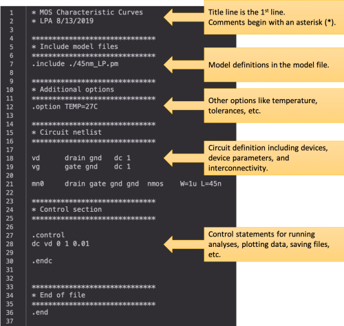
Step 2: To specify a circuit, we need to create a netlist. The netlist describes the devices, their parameters, and how they are interconnected. In this example, we will use this netlist:
Take note of the following instantiation format:
Voltage source instantiation:
vx..x <positive terminal> <negative terminal> <parameters>
MOSFET instantiation:
mx..x <drain> <gate> <source> <body> <model name> <parameters>
Step 3: The ngspice simulator can be invoked from the terminal command line via:
$ ngspice
This brings up the simulator in interactive mode, and you are presented with a prompt:
ngspice 1 ->
Step 4: To load our circuit netlist named mos_characteristics.sp, we type in the command at the ngspice prompt:
ngspice 1 -> source mos_characteristics.sp

Circuit: * mos characteristic curves

Doing analysis at TEMP = 27.000000 and TNOM = 27.000000


No. of Data Rows : 101

ngspice 2 ->
Note that the simulator has performed the analysis we have specified in the control section of the input netlist: a DC analysis, sweeping the voltage source vd from 0V to 1V, in steps of 0.01V.
Step 5: We can view the output graphically via the command:
ngspice 2 -> plot -i(vd)
The term -i(vd) specifies that we want to plot the current flowing out of the positive terminal of the voltage source vd. A negative sign is added since, by convention, the positive current is defined as the current into the positive terminal of the voltage source.
A window, showing the value of the transistor drain current (negative of the current into the positive terminal of vd) as the drain voltage is varied, is opened.
If we want to print the simulation result as a table of values and write it to a file mos_characteristics.dc, either for further post-processing or for other types of visualizations, we can use:
ngspice 3 -> print -i(vd) > mos_characteristics.dc
Or alternatively, if you want to tabulate the results without the table headers, you can use:
ngspice 4 -> wrdata mos_characteristics.dc -i(vd)
Step 6: Transistor parameters such as small-signal parameters (taken at the calculated DC operating point) and model parameters can be read using the following commands:
ngspice 5 -> print @mn0[vth]

ngspice 6 -> print @mn0[gm]

ngspice 7 -> print @mn0[id]

ngspice 8 -> print @mn0[cgg]
You may consult the ngspice manual for a list of accessible parameters.
Exercise
Characterize both nmos and pmos of the same technology. Compare their (1) Ion, Ioff, and their ratio; (2) threshold voltage; and (3) gate capacitance.
